-
LADSIM
 View
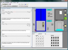
ViewLADSIM is a fully functional ladder logic design and PLC simulation software program that incorporates the functions used in PLC ladder programming. LADSIM uses the PC as a virtual PLC.
LADSIM includes a visual editing environment for graphical programming. A simple ‘drag and drop’ method is used to add functions to the ladder rung, and comments can be added to each rung for documentation purposes. LADSIM functions include inputs, outputs, timers, counters, flags and shift registers. An interactive debugger is included allowing the program to be tested before being used to control a specific application.
LADSIM has eight internal simulations; Annunciator, Traffic Light, Car Park, Elevator, Drinks Machine, Packing Line, Bottling Plant, and the ICT3. Each simulation is designed to aid and test knowledge of programming in ladder logic.
LADSIM has the ability to be connected to external devices, through a suitable interface. The student can start with the internal simulations and then move onto the ICT3 simulation once completed it is then possible to connect an actual ICT3, using an interface card and control this through the real I/O. The courseware begins with a general introduction to PLCs, the various programming methods available and the fundamentals of ladder logic programming and then moves onto the functions of LADSIM. Developing programs to monitor and control each of the simulations is part of the curriculum coverage.
-
PCUSIM
 View
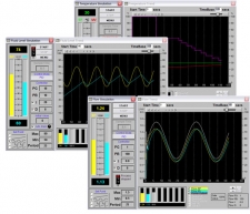
ViewPCUSIM is a simulation software used to teach process control. The program is aimed at further and higher education students learning process engineering and process control using Three Term Control (PID) methods.
PCUSIM has a graphical display of all data in real time. Graphs can be analysed, rewound, saved and printed. Experiments for flow, level, temperature and batch can be performed. Students can perform the same experiments many times with the same initial condition and different control parameters, allowing closer comparisons of outcomes.
For each of the control screens in flow, level, temperature and batch, displays show : start and stop buttons, the control module, the principle variables being measured, PID parameters, set-point; real-time graph with start time and time base, state of current reading and reading being examined with tick boxes for each traces to displayed.
Courseware manual and build in help files provided to allow students to proceed without full time supervision.
-
WinCODAS
 View
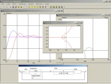
ViewWinCODAS is an application for Control System Design using a Multiple Document Interface (MDI) which allows an arbitrary number of child windows to be created. In each child window the behaviour of a system may be examined in different ways. WinCODAS allows time and frequency responses to be drawn. There is a root domain where root-loci may be plotted either in the s-plane or z-plane.
Nonlinearities may be defined in a flexible and simple manner and their characteristics drawn. These nonlinearities can then be included into the control loop simulation. Time domain responses may be drawn as phase-plane diagrams. A wide range of cost-functions may be defined, settling time, integral of error squared. The cost-functions are evaluated automatically when a response is produced. The frequency domain supports direct and inverse Nyquist diagrams, Bode gain and phase plots and Nichols plots. Closed-loop gain contours (M-contours) may also be drawn. The root domain shows the open-loop poles and zeros of the system and draws root-loci for continuous-time systems with or without transport delay and discrete-time systems. Damping-ratio or Jury contours may be superimposed on a root locus diagram. For rational transfer functions, the positions of all the closed-loop poles may be displayed in a table and marked on the root locus plot.
A digitised cursor is available in all domains to obtain details of data on any plot. The cursor can be switched from absolute to relative mode to allow relative measurements such as peak overshoots or the period of an oscillatory response. There is an auto-scale function and a zoom feature that allows users to magnify any section of a plot. Each child window can have multiple plots; none of which are lost when the window is resized. The system transfer functions are entered in “free-format”. Continuous-time, discrete time and sampled-data systems may be simulated by defining the appropriate transfer function and sample hold time. There are several mapping tools that allow the user to transform transfer functions into explicit z-domain representations including: zero-order hold z-transform, rectangular rule, Tustin’s rule with pre-warping and there are a number of manipulation tools for changing the presentation of the transfer functions into Bode form, pole/zero form. The simulated system is shown graphically in a separate window and its configuration can be different for each child window. As a child window is brought into focus, the system graphic changes dynamically and so the user knows the precise nature of the system being simulated. The general system includes an overall system gain, two transfer functions, a transport delay, two nonlinearities and a zero-order hold. These elements can be included or excluded. There are three possible inputs to the system. In this way the regulation behaviour due to load disturbances and measurement noise can be simulated as well as the performance with more standard set-point or reference inputs.